SPaircraft 101
These instructions will help you run SPaircraft for the first time!
SPaircraft.py - set of aircraft models
SPaircraft.py contains a set of methods that are used to optimize different aircraft configurations.
The process to create and run one of these models is general. The following definitions are required:
- Nclimb, number of climb segments
- Ncruise, number of cruise segments
- Nmission, number of missions to simulate
- objective, which is a string designating the objective function
- aircraft, which is a string designating the type of aircraft
The following imports are also required:
import numpy as np

# GPkit tools
from gpkit import units, Model
from gpkit import Variable, Model, units, SignomialsEnabled, SignomialEquality, Vectorize
from gpkit.constraints.bounded import Bounded as BCS

# Constant relaxation heuristic for SP solve
from relaxed_constants import relaxed_constants, post_process

# Mission model
from aircraft import Mission
For the demonstration, we define these as:
Nclimb = 3
Ncruise = 2
Nmission = 1
objective = 'W_{f_{total}}' # minimizing fuel burn
aircraft = 'optimalD8' # optimizing the optimalD8 configuration
Now, we have the basic building blocks of a model:
m = Mission(Nclimb, Ncruise, objective, aircraft, Nmission)
Since we are optimizing a D8.2 aircraft, we need to import the appropriate parameter substitutions:
from subs.optimalD8 import get_optimalD8_subs
substitutions = get_optimalD8_subs()
And we need to specify a mission range and number of passengers:
substitutions.update({'R_{req}': 3000.*units('nmi'),
                      'n_{pass}': 180.})
We can update our model m with the substitutions:
m.substitutions.update(substitutions)
m = Model(m.cost, BCS(m))
We use Bounded (BCS) in SPaircraft to make sure that the models are stable even if not all variables are well-constrained. Users are warned about unbounded variables at the end of the solve.
We implement the relaxed constants heuristic to solve the SP:
m_relax = relaxed_constants(m, None)
Now we solve, and print the results:
sol = m_relax.localsolve(verbosity=4, iteration_limit=200, reltol=0.01)
print sol.table()
Congratulations!
Solution visualization
We implement an integration with OpenVSP to show the outer mold line (OML) of each aircraft configuration after they are optimized with SPaircraft. To be able to use this functionality, the users needs to download and install the OpenVSP software, which is available here.
Once OpenVSP is successfully installed, the .vsp3 files in the VSP directory will be recognized and accessible. Clicking any of these will open up the OpenVSP interface, which looks similar to this:

As an example, to be able to visualize the optimized D8.2 aircraft within our solution sol, we import the following functions in the Python console:
# VSP visualization tools
from saveSol import updateOpenVSP, gendes, gencsm
We currently support both openVSP and ESP. openVSP is used purely for visualization, and ESP outputs will have the capability to be used for highfidelity simulations in the future. To generate the required files, type this into the console:
gendes(m, sol, 'optimalD8', 0) # Generates design0.des Design Variables file within the **VSP**  directory for openVSP.
gencsm(m, sol, 'optimalD8', 0) # Generates d82-0.csm file within **ESP** directory for ESP serveCSM.
To load this .des files, click File, and select Run Script…. In the pop-up, select reload.vspscript. To load ESP files, once you have ESP installed and its environment ready, call serveCSM on the .csm file and voila! You have generated the OML of the D8.2 aircraft.
Static vs. Performance Models
To allow for multipoint aircraft optimization over multiple flight segments, missions, or loading cases, two models are created for each aircraft component - a static and a performance model. The static model contains all variables and constraints that do not change between operating points, such as component weights and dimensions. Performance models contain all constraints and variables that change between operating points, such as air speeds, lift coefficients, and fuel quantities. To simulate multiple aircraft missions, the performance models and the static variables that change between missions (eg. number of passengers and fuel weight) are vectorized. When a model is vectorized, all the variables it contains become vectors, with each element corresponding to a different operating point. Figure 1 provides a visual representation of static and performance models.
Model hierarchy
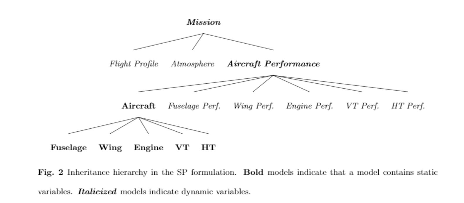
The SP formulation develops implements a hierarchy in optimization parameter and variable definitions, due to the serial nature of software engineering tools. This hierarchy is shown in Figure 2, where each higher level in the framework inherits the variables, parameters, and constraints in the layers below.
Single- vs. multi-mission optimization
A user can switch between the two modes by modifying the Nmissions variable above, or within the optimize_aircraft function. Note that you will have to modify the objective function, and the substitutions for range and passengers to match the number of missions you would like to consider. This will optimize a given configuration over a set of missions.